Diagnostic plots for `tspa` models

Jimmy Zhang

2024-09-06

The example is from https://lavaan.ugent.be/tutorial/sem.html.

Load packages

library(lavaan)
library(R2spa)

Single group, single predictor

model <- ' 
  # latent variable definitions
     ind60 =~ x1 + x2 + x3
     dem60 =~ y1 + a*y2 + b*y3 + c*y4

  # regressions
    dem60 ~ ind60
'

fs_dat_ind60 <- get_fs(data = PoliticalDemocracy, 
                       model = "ind60 =~ x1 + x2 + x3")
fs_dat_dem60 <- get_fs(data = PoliticalDemocracy, 
                       model = "dem60 =~ y1 + y2 + y3 + y4")
fs_dat <- cbind(fs_dat_ind60, fs_dat_dem60)

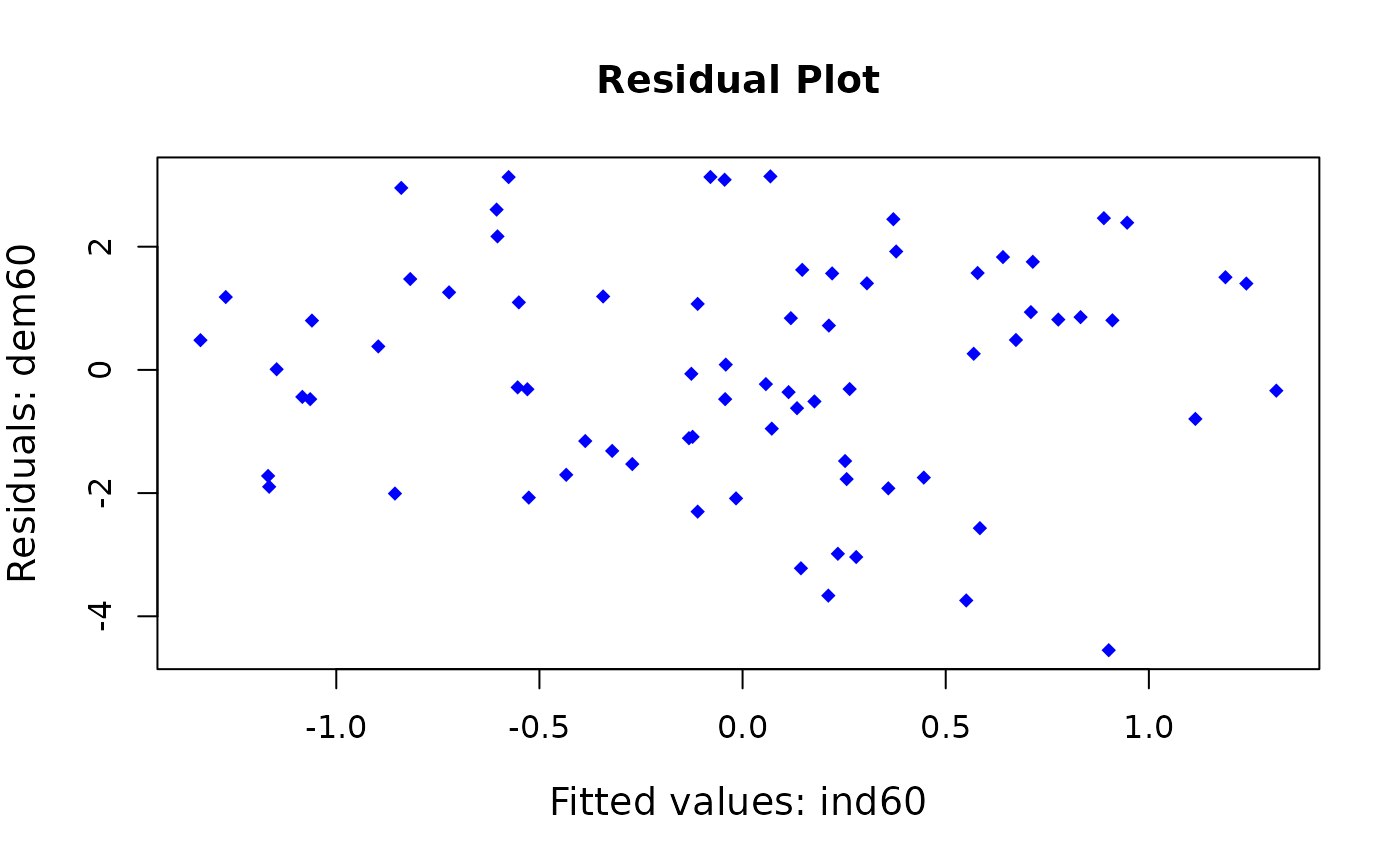
tspa_fit_1 <- tspa(model = "dem60 ~ ind60", 
                   data = fs_dat, 
                   se_fs = list(ind60 = 0.1213615, dem60 = 0.6756472),
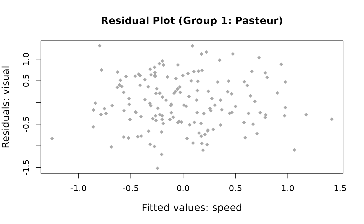
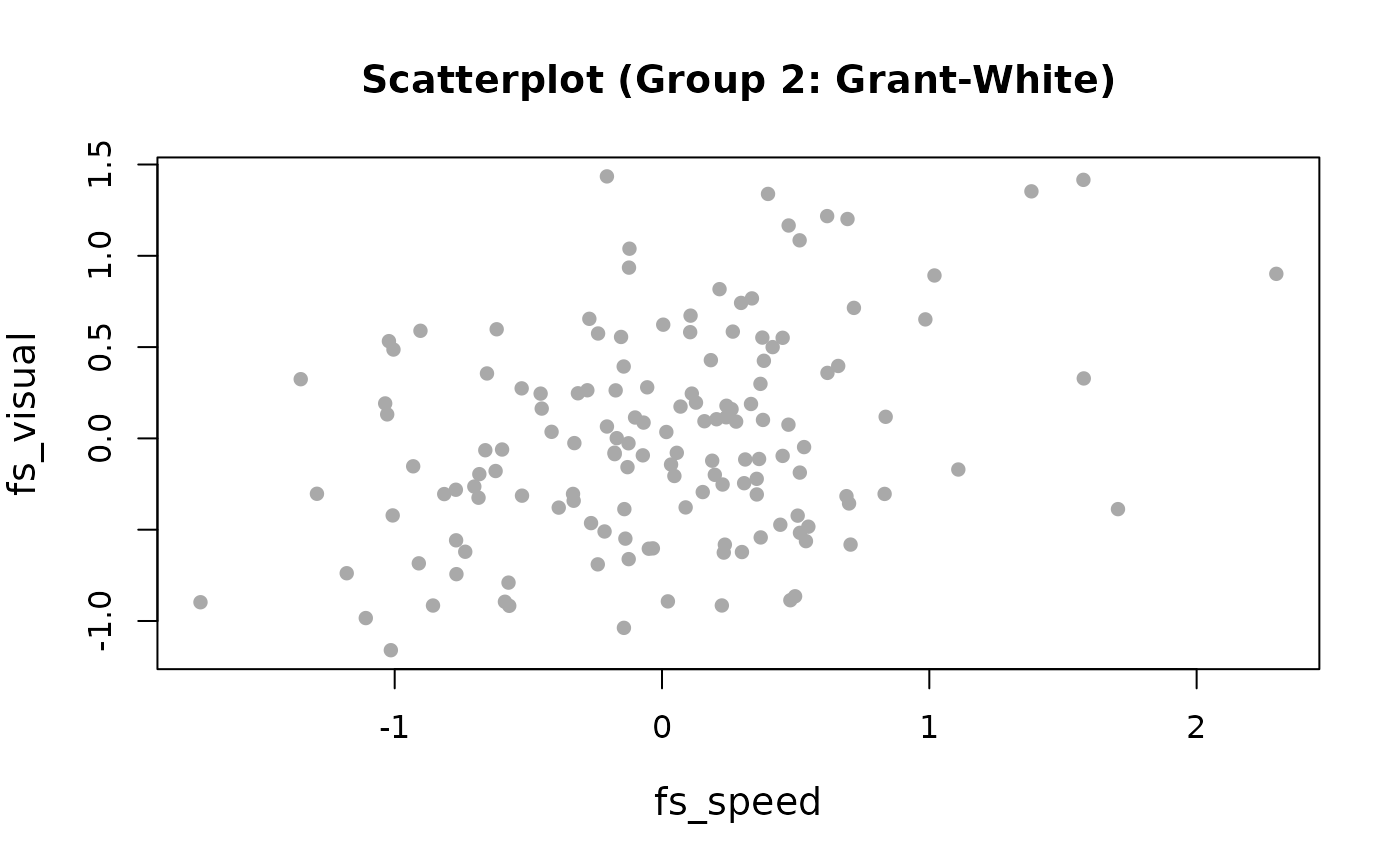
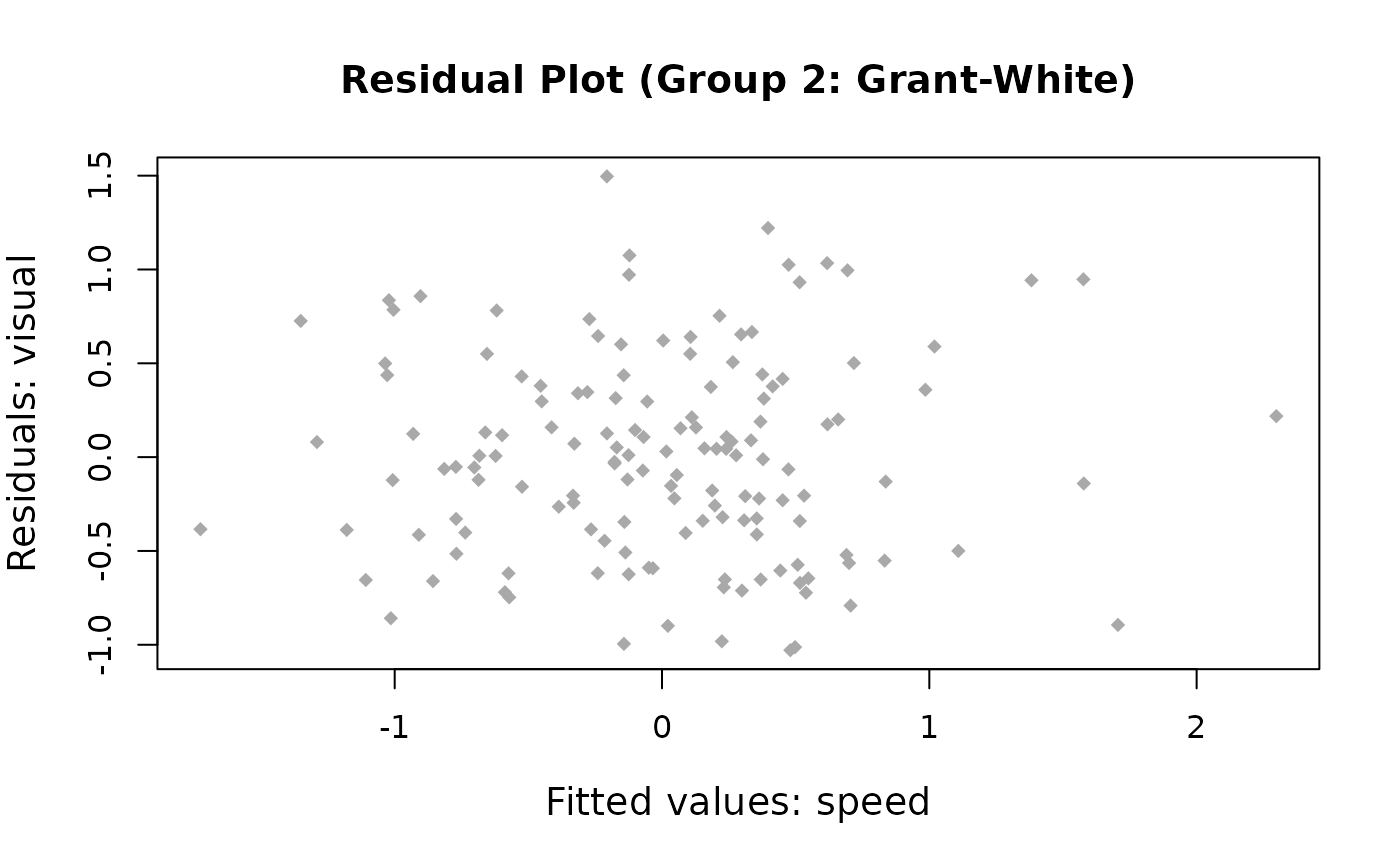
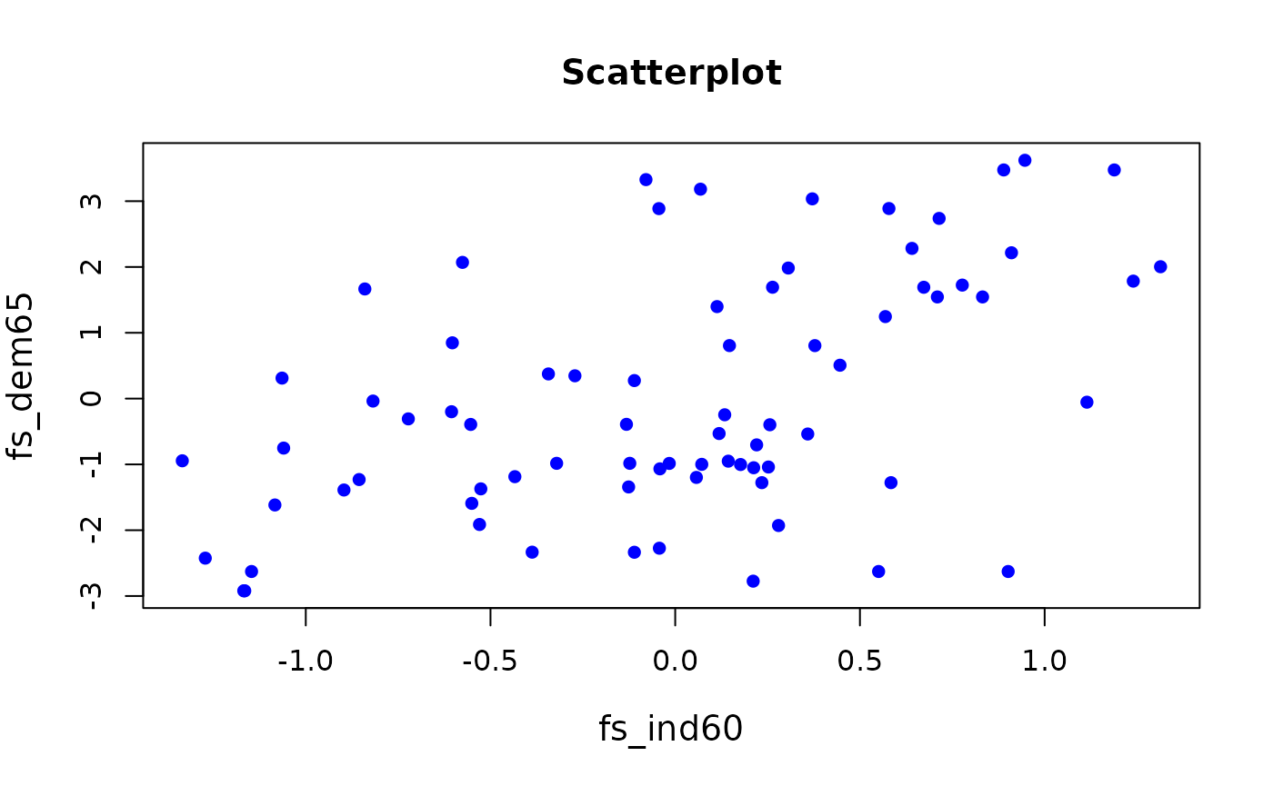
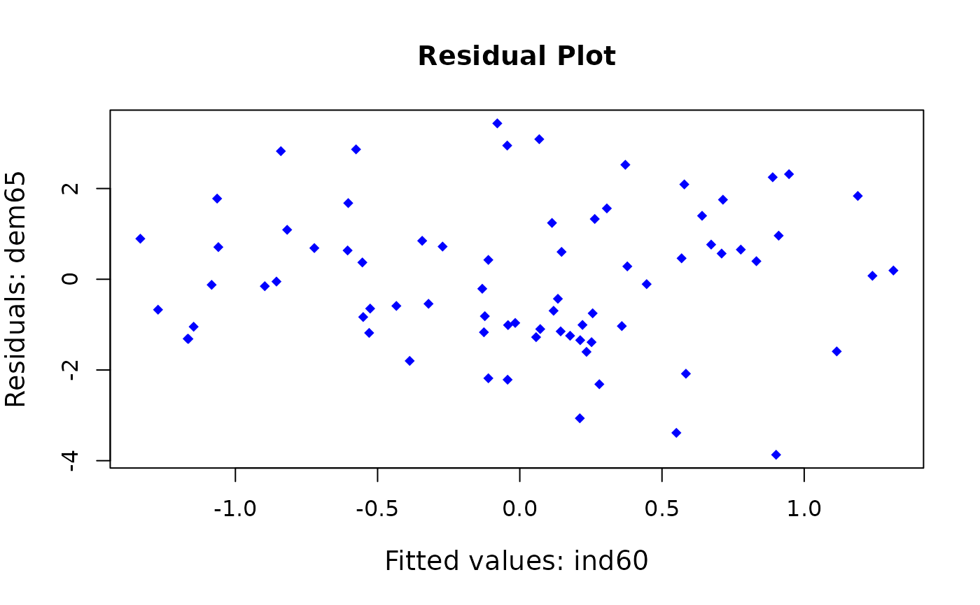
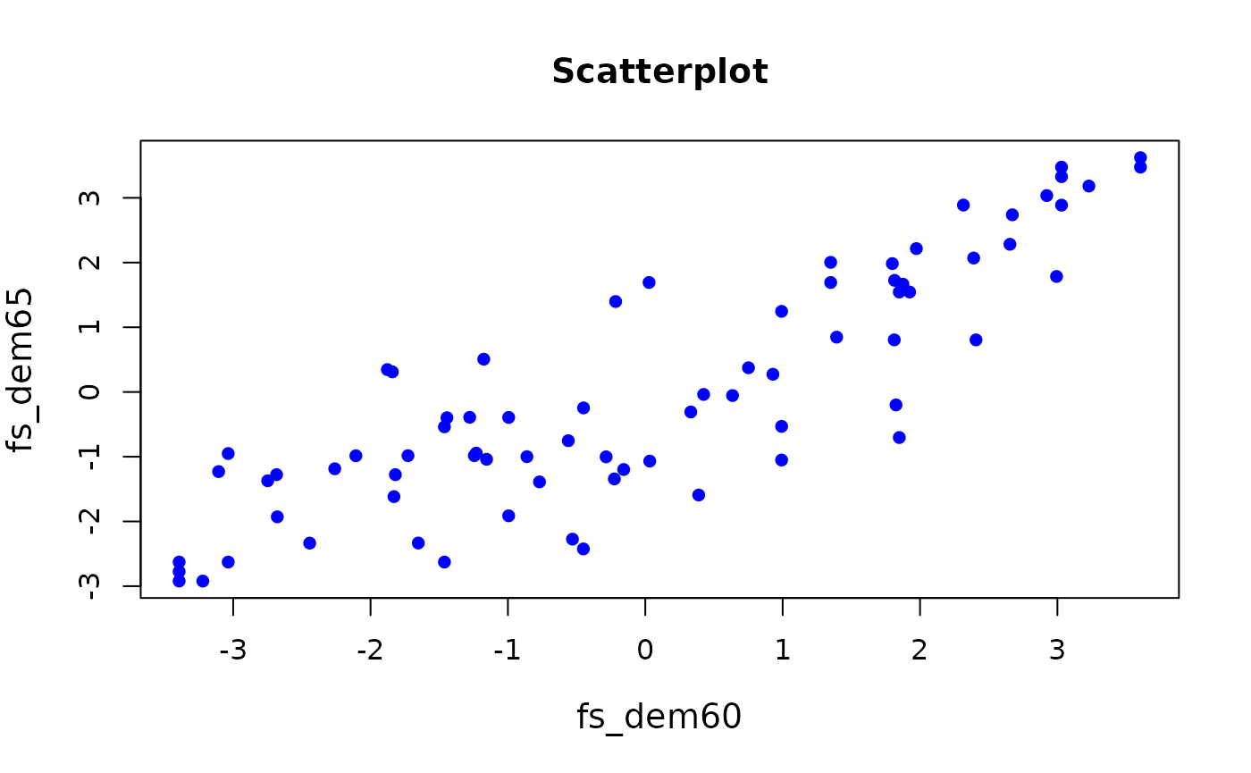
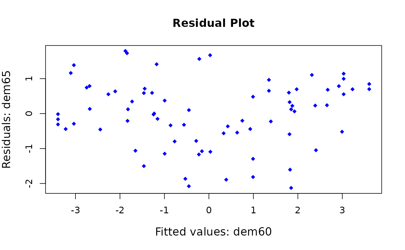
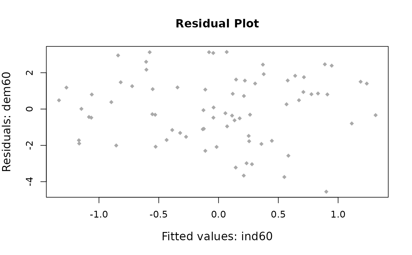
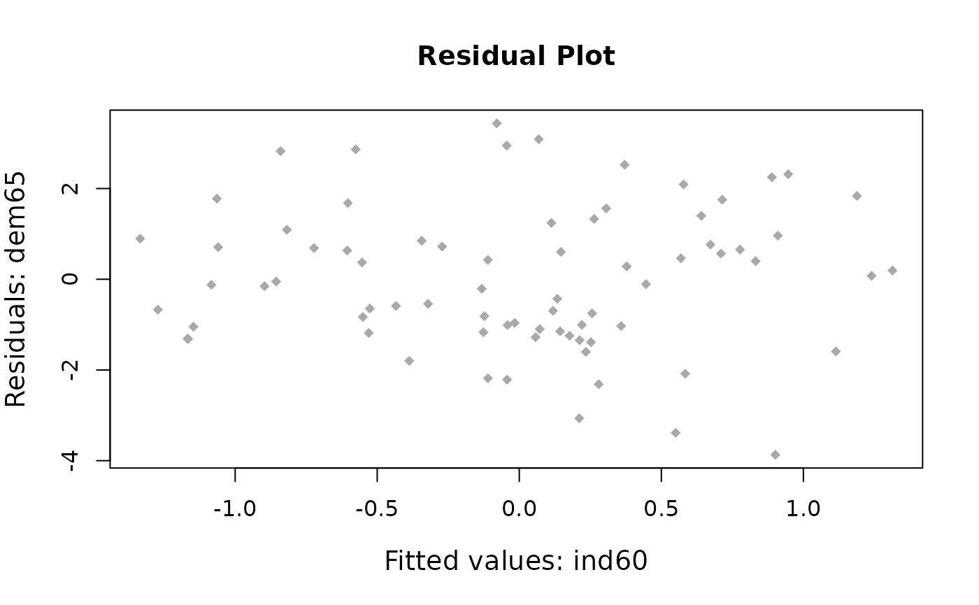
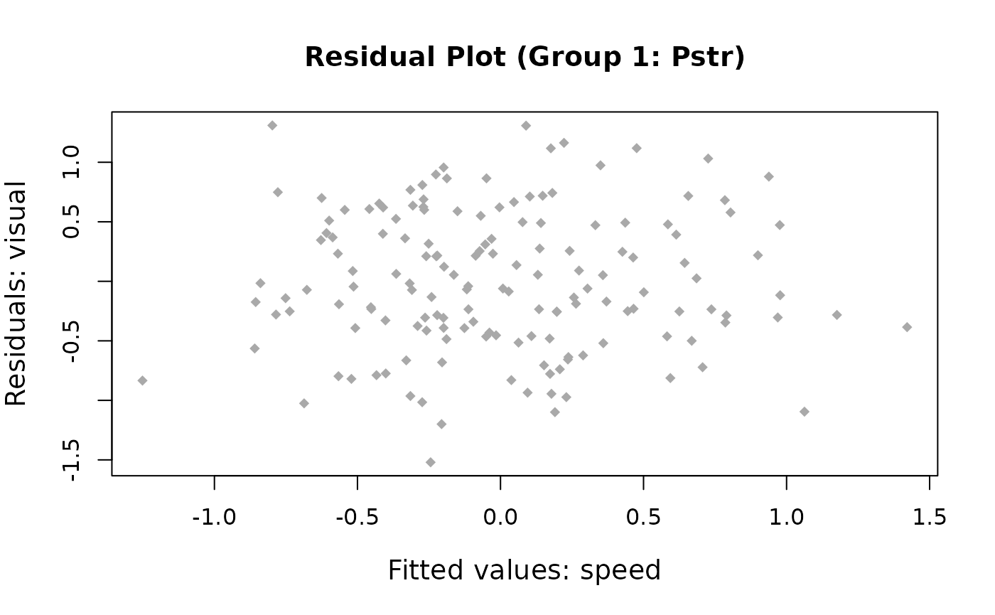
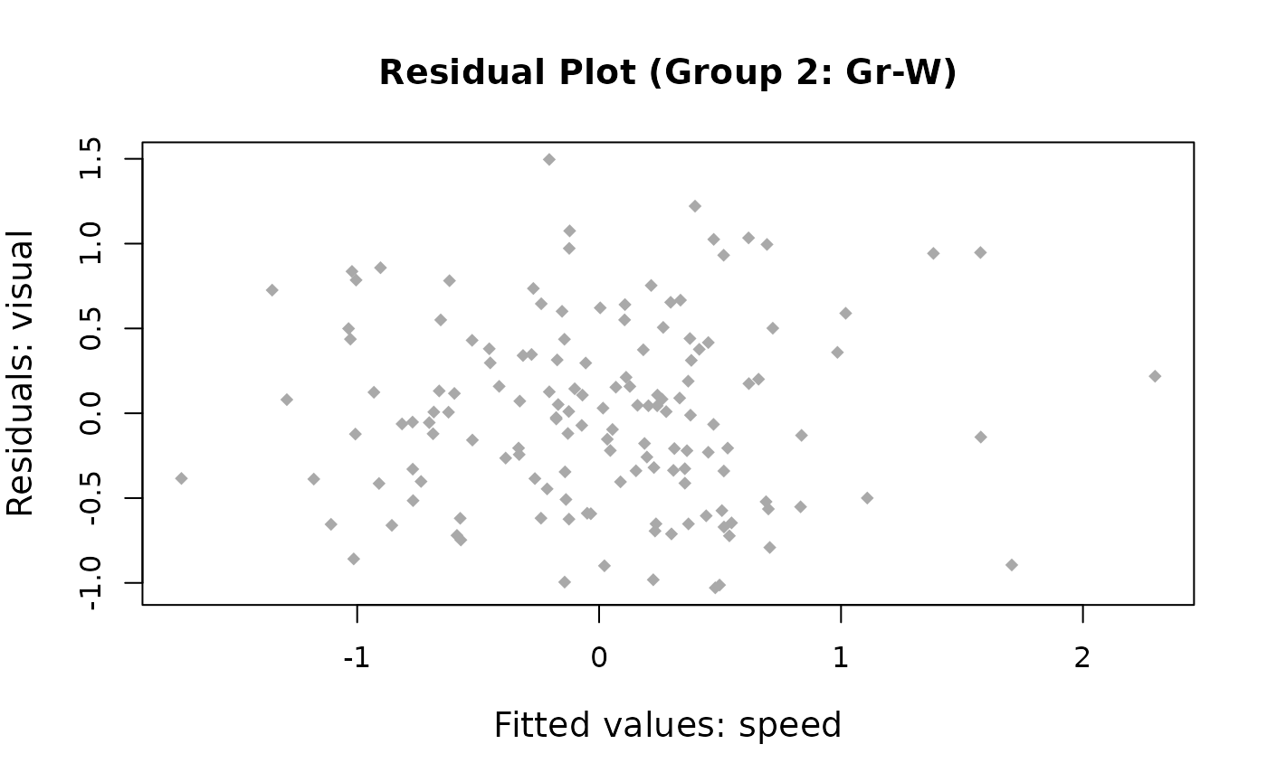
                   meanstructure = T)

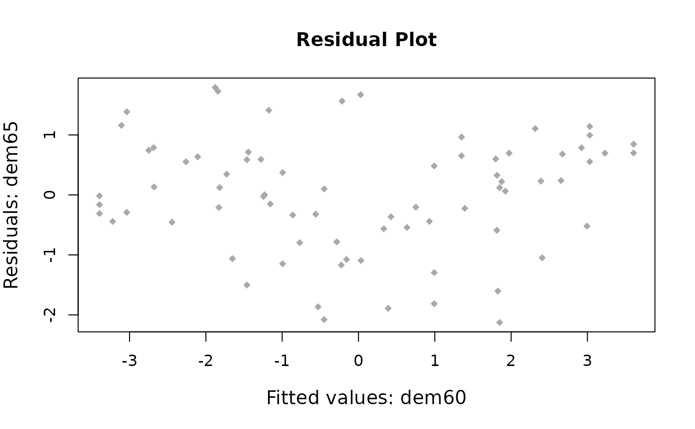
We recommend researchers to examine the diagnostic plot of factor scores in the model. They can use the function tspa_plot() to obtain two plots: (a) a scatter plot between factors, (b) a residual plot between factors.

Features of tspa_plot():

• The function is able to pass arguments to the base R plot() function.
• Users can define the title of the scatter plot and label names of axis.
• Abbreviation argument allows users to choose whether using abbreviated group names.
• Users can choose whether generating the plot one by one by hitting the on the keyboard.

# par(mar = c(2,2,3,2))
tspa_plot(tspa_fit_1,
          col = "blue",
          cex.lab = 1.2,
          cex.axis = 1,
          fscores_type = "original",
          ask = TRUE)

Using estimates from tspa() function

Single group, multiple predictors

model <- ' 
  # latent variable definitions
     ind60 =~ x1 + x2 + x3
     dem60 =~ y1 + y2 + y3 + y4
     dem65 =~ y5 + y6 + y7 + y8

  # regressions
    dem60 ~ ind60
    dem65 ~ ind60 + dem60

  # # residual correlations
  #   y1 ~~ y5
  #   y2 ~~ y4 + y6
  #   y3 ~~ y7
  #   y4 ~~ y8
  #   y6 ~~ y8
'

fs_dat_ind60 <- get_fs(data = PoliticalDemocracy, 
                       model = "ind60 =~ x1 + x2 + x3")
fs_dat_dem60 <- get_fs(data = PoliticalDemocracy, 
                       model = "dem60 =~ y1 + y2 + y3 + y4")
fs_dat_dem65 <- get_fs(data = PoliticalDemocracy, 
                       model = "dem65 =~ y5 + y6 + y7 + y8")
fs_dat <- cbind(fs_dat_ind60, fs_dat_dem60, fs_dat_dem65)

tspa_fit_2 <- tspa(model = "dem60 ~ ind60
                            dem65 ~ ind60 + dem60", 
                   data = fs_dat, 
                   se_fs = list(ind60 = 0.1213615, dem60 = 0.6756472, 
                                dem65 = 0.5724405))

# Title, xlab, and ylab each with same names.
tspa_plot(tspa_fit_2,
          ps = 10,
          col = "blue",
          cex.lab = 1.2,
          cex.axis = 1)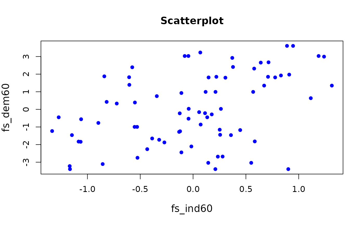

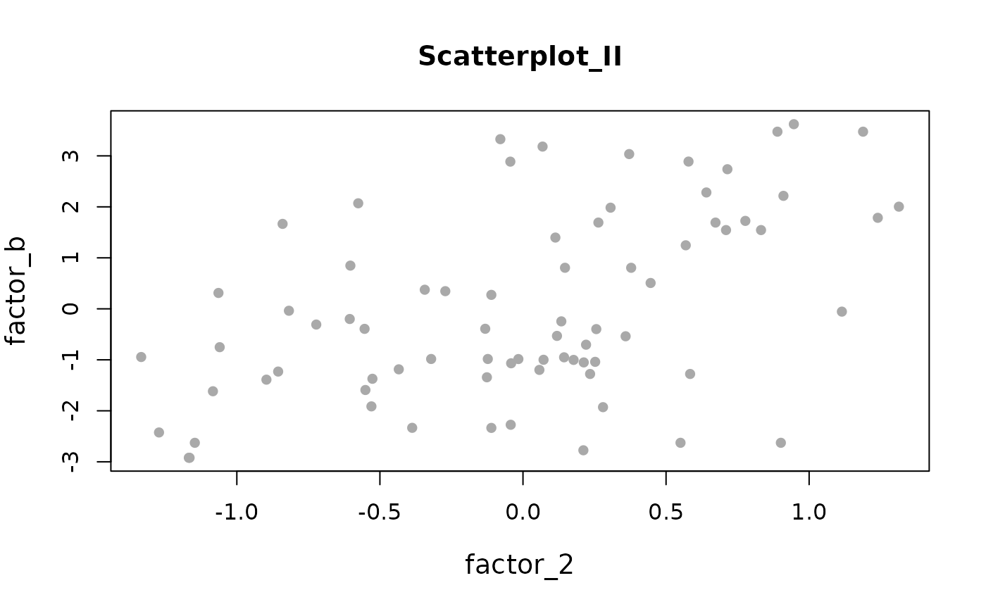
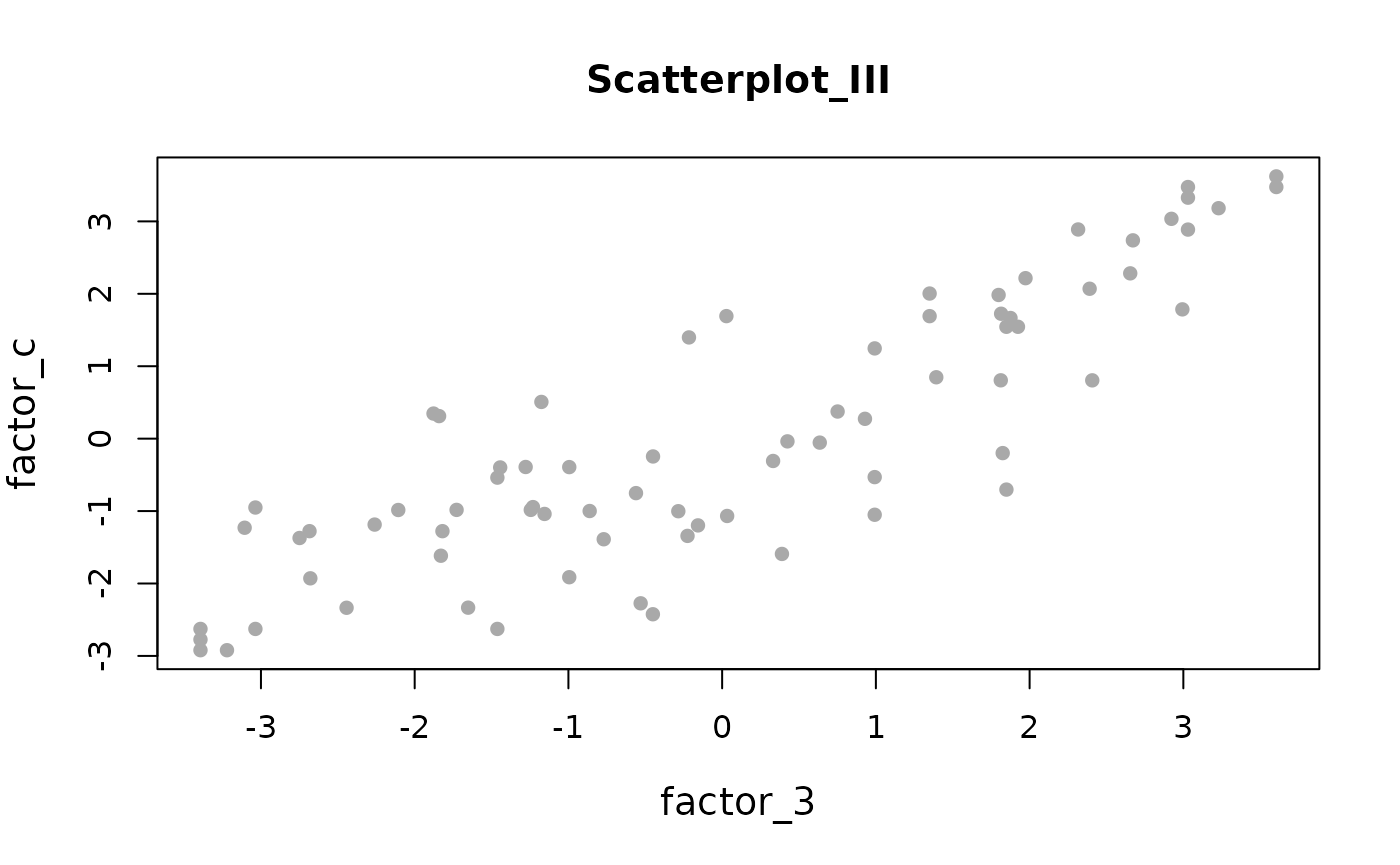
# Title, xlab, and ylab each with separate names.
tspa_plot(tspa_fit_2,
          ps = 10,
          col = "darkgray",
          cex.lab = 1.2,
          cex.axis = 1,
          title = c("Scatterplot_I", "Scatterplot_II", "Scatterplot_III"),
          label_x = c("factor_1", "factor_2", "factor_3"),
          label_y = c("factor_a", "factor_b", "factor_c"))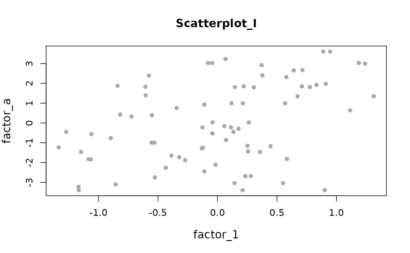

Using estimates from tspa() function

Multigroup, single predictor

model <- ' 
  # latent variable definitions
    visual =~ x1 + x2 + x3
    speed =~ x7 + x8 + x9

  # regressions
    visual ~ speed
'

# get factor scores
fs_dat_visual <- get_fs(model = "visual =~ x1 + x2 + x3",
                        data = HolzingerSwineford1939, 
                        group = "school")
fs_dat_speed <- get_fs(model = "speed =~ x7 + x8 + x9", 
                       data = HolzingerSwineford1939, 
                       group = "school")
fs_hs <- cbind(do.call(rbind, fs_dat_visual),
               do.call(rbind, fs_dat_speed))

tspa_fit_3 <- tspa(model = "visual ~ speed",
                   data = fs_hs,
                   se_fs = data.frame(visual = c(0.3391326, 0.311828),
                                      speed = c(0.2786875, 0.2740507)),
                   group = "school"
                   # group.equal = "regressions"
                   )

tspa_plot(tspa_fit_3,
          ps = 10,
          col = "darkgray",
          cex.lab = 1.2,
          ask = FALSE,
          cex.axis = 1)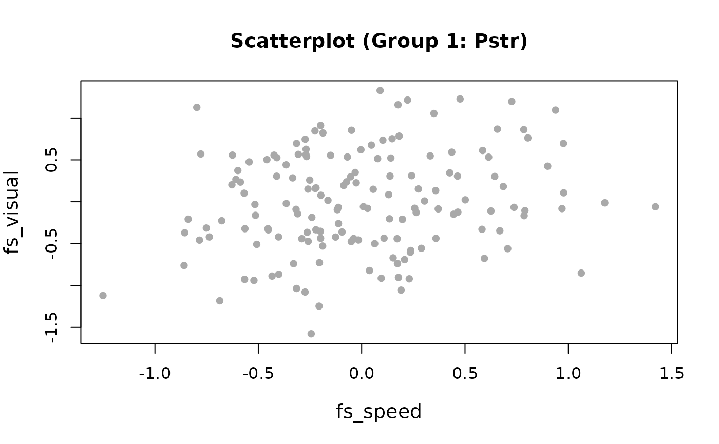

tspa_plot(tspa_fit_3,
          ps = 10,
          col = "darkgray",
          cex.lab = 1.2,
          cex.axis = 1,
          ask = TRUE,
          abbreviation = FALSE)